Spreadsheets offer a quick, flexible, intuitive, and cost-effective platform for rapidly analysing data and presenting information to support decision making. Spreadsheets are developed by end-users and are part of and are the most pervasive example of the End User Computing (EUC) group of applications that form a bridge between the non-IT business requirements and the stringently managed IT systems. However, the fact that End-Users are not subject to the same controls prevalent in IT systems have led to increased risks for many of the businesses that rely on them.

Spreadsheets are rarely a cause for concern or suspicion. Management may believe there is little reason for concern because they have used the same spreadsheet software for many years, even though they should be. Spreadsheets can easily be changed, may lack certain controls, and are vulnerable to human error.

According to research, 95% of spreadsheets contain errors! The risks from Spreadsheet errors has caused many businesses to lose revenue and profit or find their reputation damaged as a result of spreadsheet error.

ExcelAnalyzer software uses state-of-the-art algorithms to help users resolve errors and risks, and gain confidence in their spreadsheet results again, by combining powerful error detection with investigative capabilities to comprehensively analyse spreadsheets. ExcelAnalyzer reduces material errors and possible fraud as well as the hours associated with detailed spreadsheet review.

ExcelAnalyzer scans spreadsheets for likely errors and inconsistencies and uses powerful algorithms to identify them for investigation and possible correction if found to be errors. It identifies these errors and risks quicker and more extensively than any other solution.

The speed with which ExcelAnalyzer allows the User to review, audit and correct the errors and inconsistencies in a matter of minutes, saves huge amounts of time and money compared with manual processes. This also eliminates the commercial, financial and reputational risk spreadsheet errors can cause.

In short, ExcelAnalyzer will help you to check your Excel files and feel secure that the Spreadsheet used is correct.

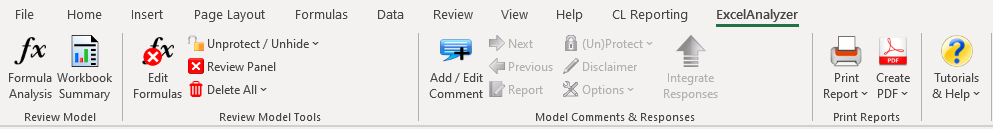
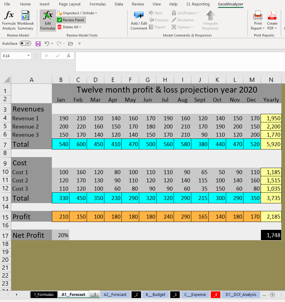
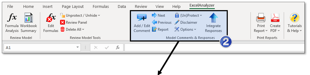
Above is the ExcelAnalyzer Ribbon.

ExcelAnalyzer provides a number of powerful features to review and audit any spreadsheet from the smallest single sheet spreadsheet to the largest complex multi-sheet model:

• Formula Analysis
• Workbook Summary – Detailed Report
• Workbook Summary – Model Flow Report
• Workbook Summary – General Report
• Comment Feature

Formula Analysis

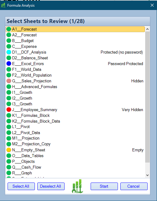
The Formula Analysis process starts by displaying the following that shows the name and status of each sheet and allows you to select individual sheets or all sheets to review and audit. Hidden and Protected sheets must be Un-Hidden and Unprotected to be included in the review process. Empty sheets are not reviewed.

As well as providing a Formula Analysis report, this powerful feature generates a copy of each original sheet which it puts next to each original sheet. It also gives a different colour to each unique formula on each sheet.

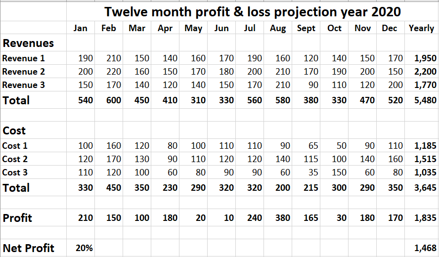
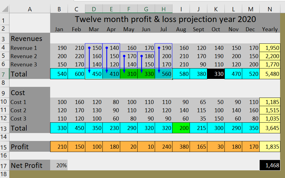
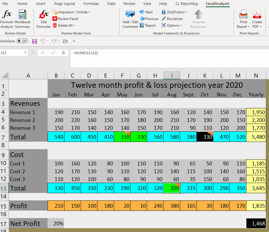
This copies the original sheet turning it from this:

To this:

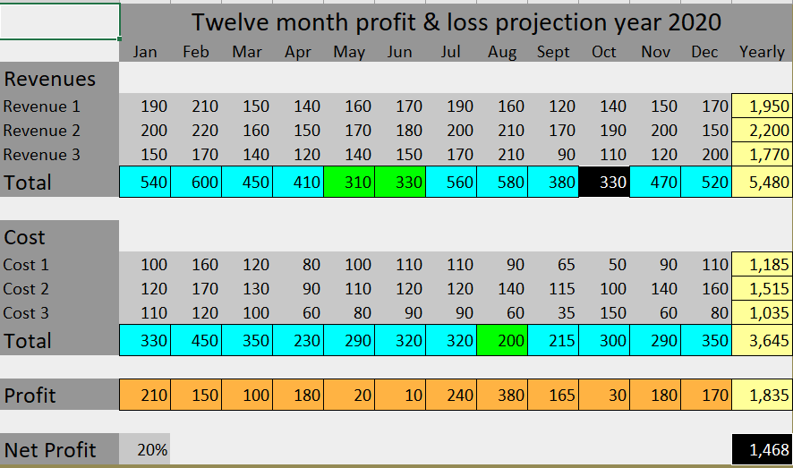
Which clearly displays, in seconds, the inconsistencies to investigate since each different colour represents a unique formula. The cells with a green background and a black background amongst the cells with a blue background instantly standout for investigation since it means they have a different formula to the blue background cells.

On the right of each copied sheet content is the Review Panel that contains features to conduct an additional detailed in-depth investigation of the sheet.

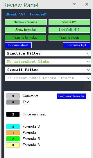
For instance, by using the “Tracing Formulas” button in the Review Panel you can display the components of the formulas as is shown below:

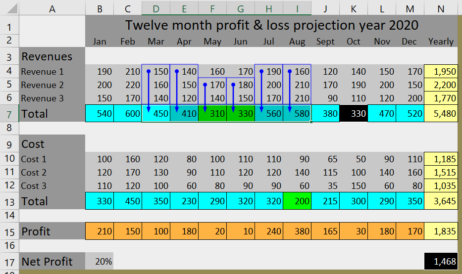
This clearly shows that the formulas in cells F7 & G7 have both omitted a cell from the SUM functions. To correct this,

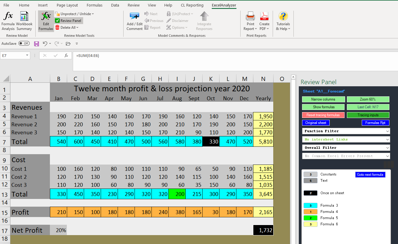
You must first click on the Edit Formulas button in the ExcelAnalyzer ribbon which unprotects this copied sheet and replicates any changes to the original sheet. Next select cell E7 and drag the handle (shown at the bottom right corner of the cell by the blue arrow) across F7 to G7 which corrects the errors as shown below.

This shows the result following the corrections to the formulas in F7 and G7.

The other 2 errors can be corrected in the same way to make this sheet error-free in just a few minutes:

Another obscure but common error that ExcelAnalyzer identifies in seconds is the following cut-and-paste error.

How long would it take you to check the following sheet?

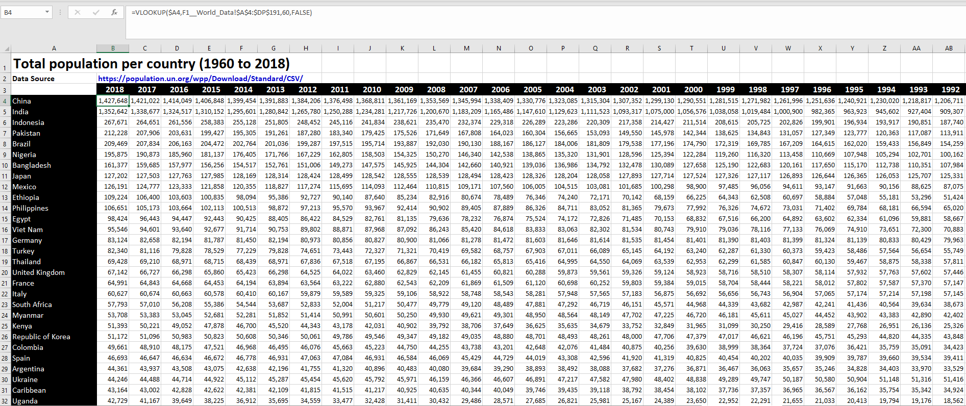
It would take many days to check each VLookup formula in each cell of this sheet. Each row’s VLookup only differs by the constant number it contains.

ExcelAnalyzer’s colour-coding makes it easy to instantly identify the errors, clearly revealing the yellow formula error block in Row G and the green block in row S, marking them for investigation and correction.

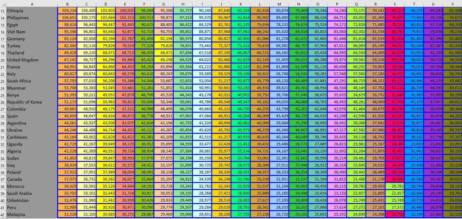
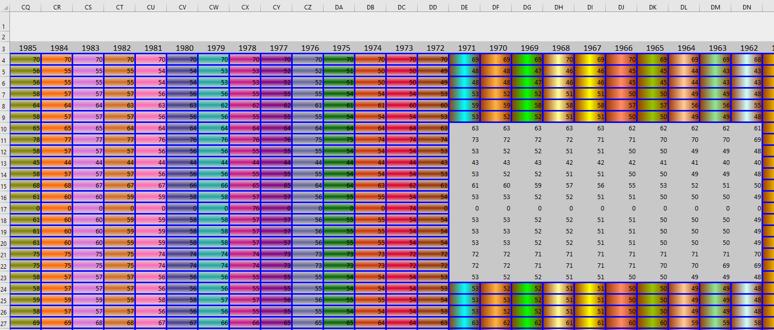
ExcelAnalyzer even identifies the cut-and-paste error below where the numbers in the box with the light-grey background have been pasted to values instead of to formulas so they contain constants instead of formulas.

So ExcelAnalyzer highlights errors and inconsistencies to allow you to quickly review, audit and correct them.

The Formula Analysis report is placed as the first tab in the sheet ribbon and contains all of the information needed to review each unique formula present in each sheet of the workbook. For convenience, all sheet names are listed and contain a link to easily

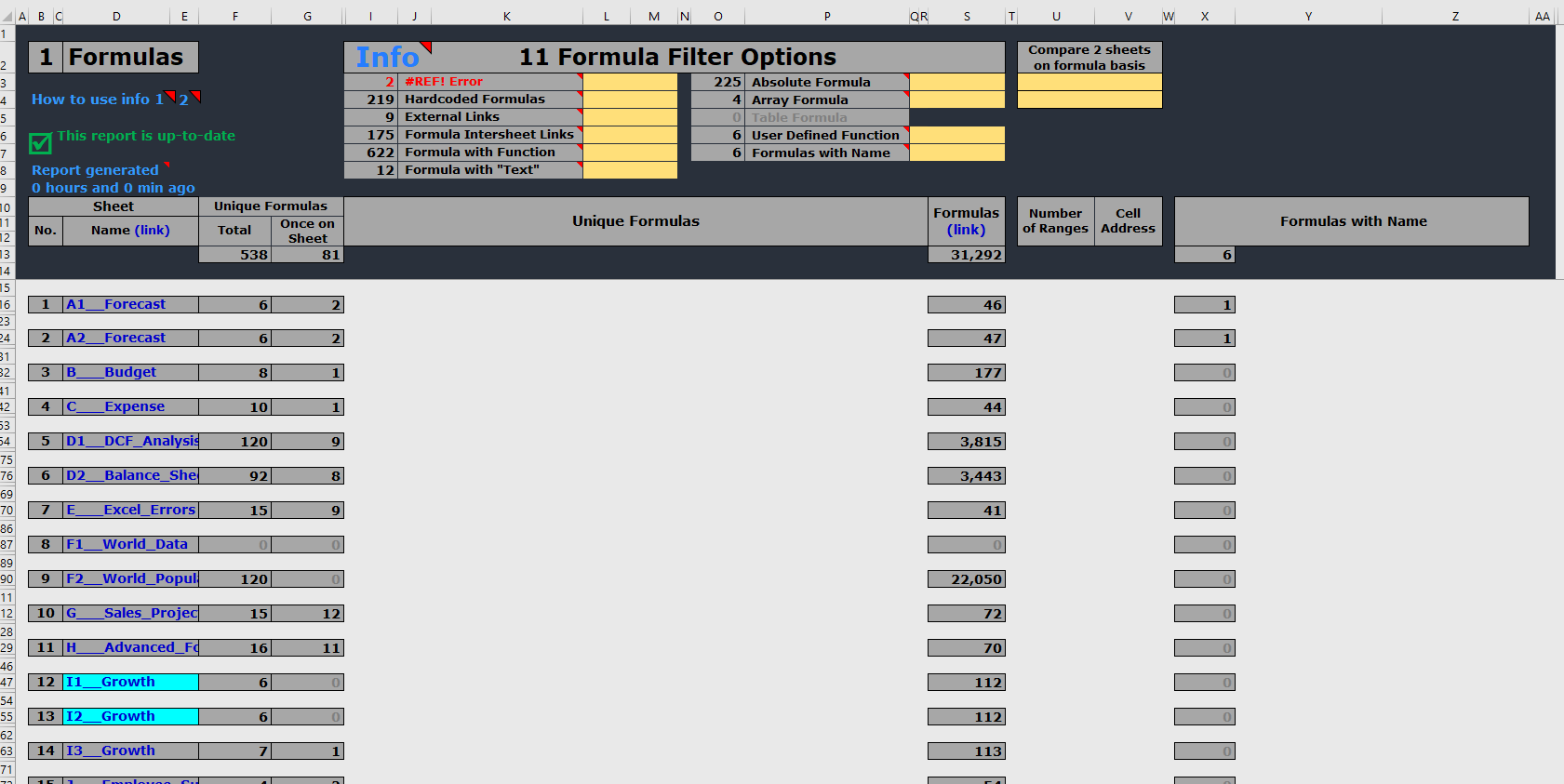
The display above shows information about each sheet including the number of formulas and unique formulas as well as a link to easily navigate and correct the issues in formulas or formula groups. It also displays how many formulas with names are on each sheet. And colour codes sheet names that have identical formulas even though they could have different text and constants.

A single click will display all of the formulas for a selected sheet or for all sheets as shown below.

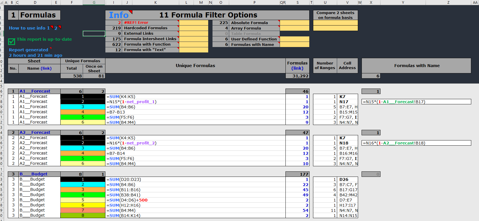
As you will see above, each formula is colour-coded to make it easier to understand and are the same colours as the ones used in the colour-coded copied sheets. So, the constant “500” stands out in sheet 3 as having been added to the formula.

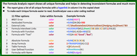
Also, the colours assigned to formulas are shown according to the following scheme which makes even the most complex formulas easier to read:

At the top of the report you will see the ability to use 11 Filter Options to drill down in more detail for each of the options such as #REF errors, hard-coded constants, external links, etc. So, for example, if you need to know precisely where a constant of “20%” is used in which formulas and in which of the 28 sheets contain those formulae, the display below shows you what you would enter in the relevant filter:

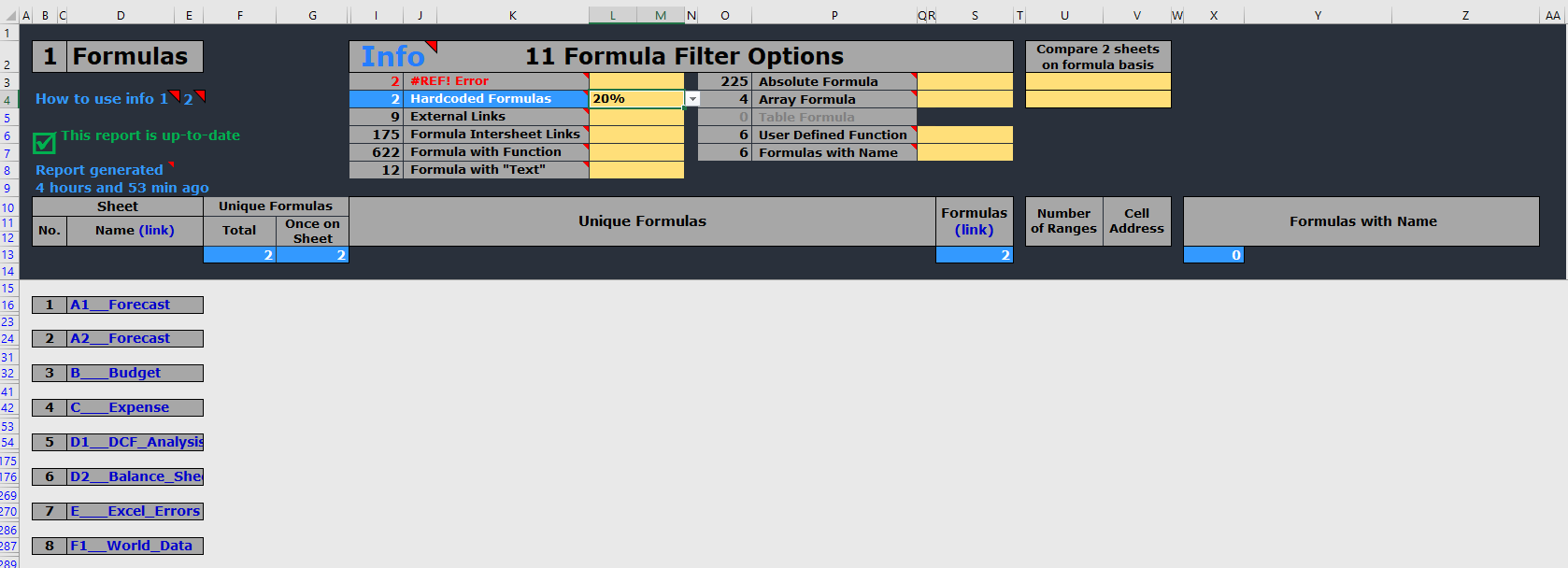
And below displays the results in seconds of searching all 28 sheets in this workbook for any formulas containing “20%”.

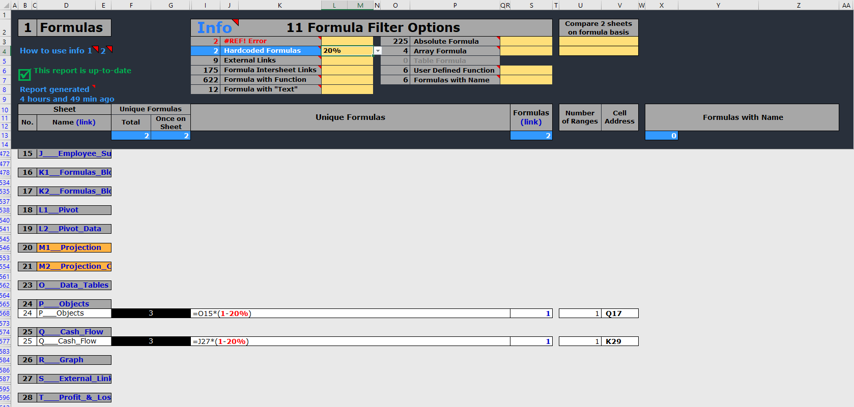
As you can see, it instantly shows the 2 sheets and the formulas containing “20%” and a link to go directly to the formula on the sheet. How long would it take you to manually search through 28 sheets to find the formulae containing “20%”?

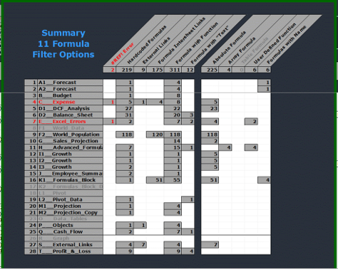
If you hover over “Info” in columns I & J you will display a summary of all of the filter options for all sheets including how many times that filter option occurs in each sheet.:

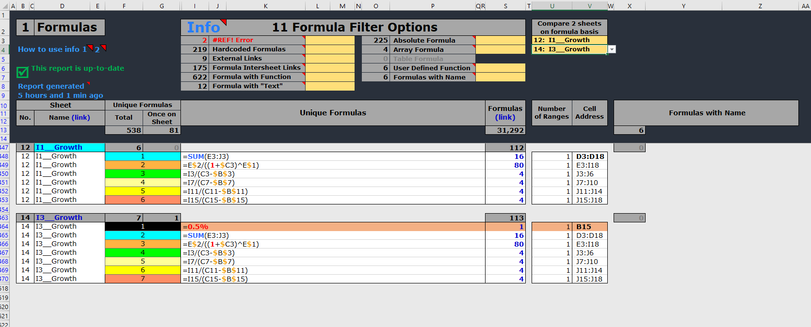
You can also compare sheets to find any differences on sheets that should have the same formulas as the Growth sheets 12,13 and 14 should have.

The sheet name colour coding shows immediately that Growth sheet 14 differs from Growth sheets 12 and 13. The display below compares sheet 14 with sheet 12 and highlights the differences which is the “0.5%” constant as shown:

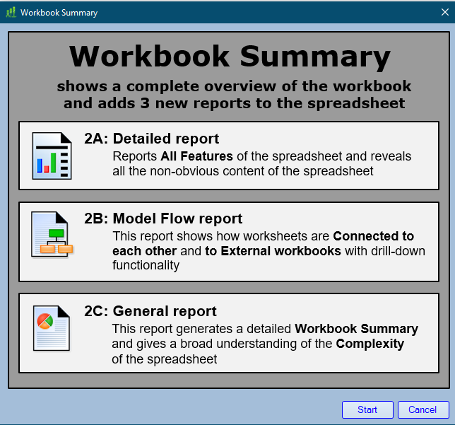
The Workbook Summary gives a complete overview of the entire workbook in three detailed reports that deal with any non-formula inconsistencies and errors since formula errors are dealt with by the Formula Analysis report:

Workbook Summary – Detailed Report

This report provides detailed information about:

• Comments
• Objects
• Hidden Columns & Hidden Rows
• Hyperlinks
• VBA Code
• Tables
• Pivot Tables
• Charts
• Conditional Formats
• Validation Cells
• Names in Formulas

This report provides the names of all VBA modules in the workbook including component names, component type, procedure names and type, start line, line count, scope, procedure declaration (hover over this entry to see the VBA code) and VBA code text without opening the VBA editor.

This report provides the sheet name and cell address with a dynamic link to the cell address. It also provides details relevant to the information being displayed. A sample display is below for Charts:

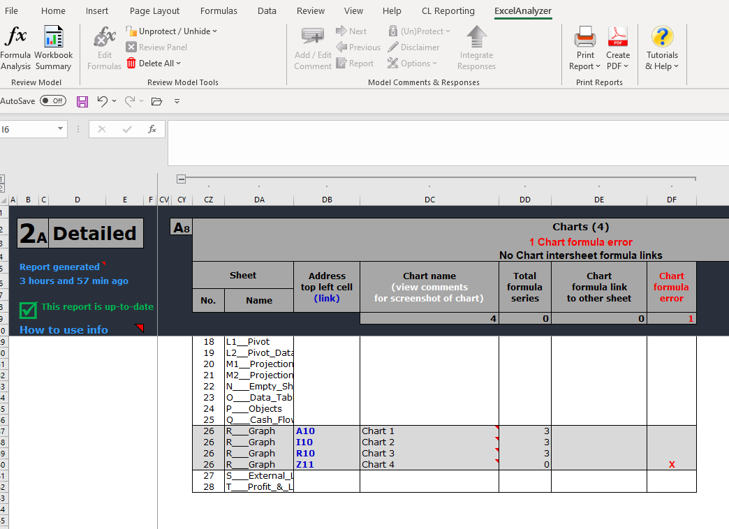
Any errors found are also flagged for investigation as can be seen in the above Chart detail and signified by the red “x”

Hovering over the chart name in question will reveal a thumbprint of that chart and then clicking on the link shown “Z11” will take you directly to that chart.

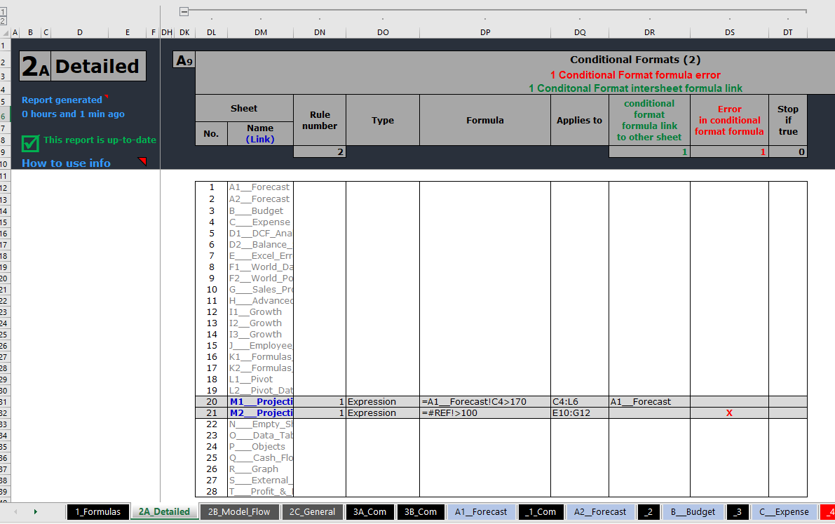
This report will also check and identify all errors such as those in Conditional Formats, showing the Conditional Format information including the sheet name, a link to that sheet, the type, the formula showing any errors and the cells the error relates to, whether there is a link to another sheet and signify the error with a red x as can be seen below

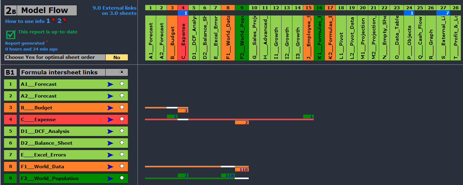
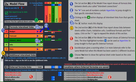
Workbook Summary – Model-Flow Report

The second of the Workbook Summary reports is the Model-Flow report. This report shows all of the links between sheets which includes the inter-sheet links and the external links. This report is particularly useful if you have a multi-sheet workbook with many links, especially if you need to delete any sheets without causing #REF errors.

The report is colour-coded and shows instantly how the sheets are connected with each other. It shows which sheets contain External Links and clicking on any of the green or orange numbered box links will navigate to that sheet and highlight those inter-sheet links and provide a link back to this report.

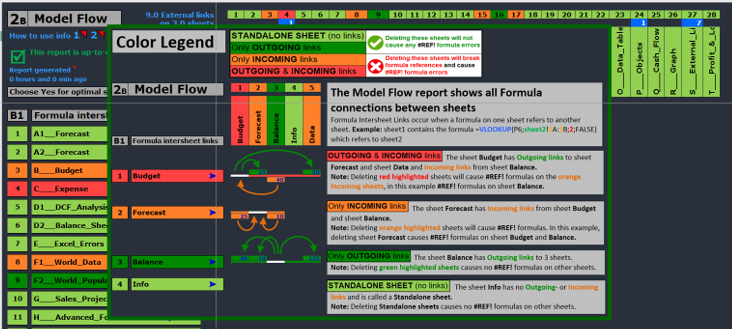
The colour-coding and links are explained in the two on-line help windows below:

This report also shows Additional Inter-sheet links and External formula links as you can see below. This report also identifies errors caused by the target of an external link being accessed from two different locations. This is probably different versions of the same link which is clearly an error.

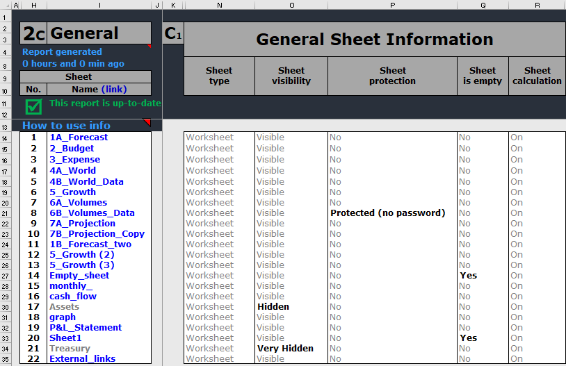
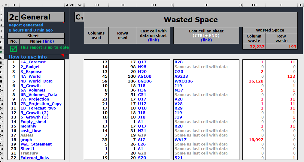
Workbook Summary – General Report

The third of the Workbook Summary reports generates a full workbook summary and gives a broad understanding of the risk level, complexity and structure of the workbook. It provides the following 4 information sections:

• General Sheet Information
• Formula Statistics
• Minimum and Maximum Values
• Wasted Space

These are shown in the following screenshots. The first section is General Sheet Information which shows the visibility and protection of sheets: is the sheet Hidden, very hidden, empty, Protected, protected with a password and whether sheet calculation is turned on or off.

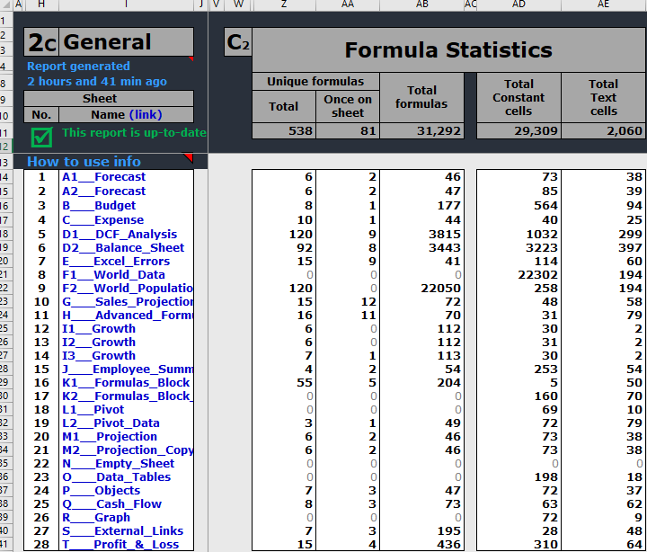
The next section is Formula Statistics. This shows the total number of formulas, unique formulas, once on a sheet formulas, total constants, and total text cells in the workbook and by each sheet. This provides the information to investigate and possibly improve the quality of the workbook by reducing the large number of formulas.

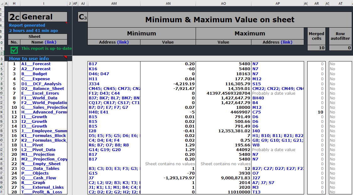
The Minimum & Maximum Value on sheet display easily identifies large positive and negative values that allow you to investigate whether they are valid:

Large, Unused sections of a sheet cause a workbook to be larger than necessary and can result in slower performance when Excel calculates formulas. This section shows you exactly how much space is unused in every sheet in the workbook and therefore how much wasted space there is in a workbook.

It shows the columns and rows used, last cell with data on the sheet, last cell on the sheet according to Excel as well as the wasted columns and rows.

The Comment Feature

The optional Comment feature is very useful for anyone who needs to review a colleague’s or a Client’s spreadsheet. Instead of the reviewer editing somebody else’s spreadsheet they can query/comment the validity of any issues in the spreadsheet and generate a comment report and send this to the model builder who can respond to the reviewer’s questions. Afterwards the reviewer or the model builder can correct the spreadsheet based on the responses of the spreadsheet owner. This option tool is accessed from section 2 of the ExcelAnalyzer ribbon.

Thus the Comment feature is a very powerful tool, not only to Review, Edit and correct the spreadsheet but also to Add Comments and therefore the comment report provides an audit trail of all issues raised in the spreadsheet by the reviewer as well as the responses provided by the model builder, Thereby documenting who changed them and how they were changed.

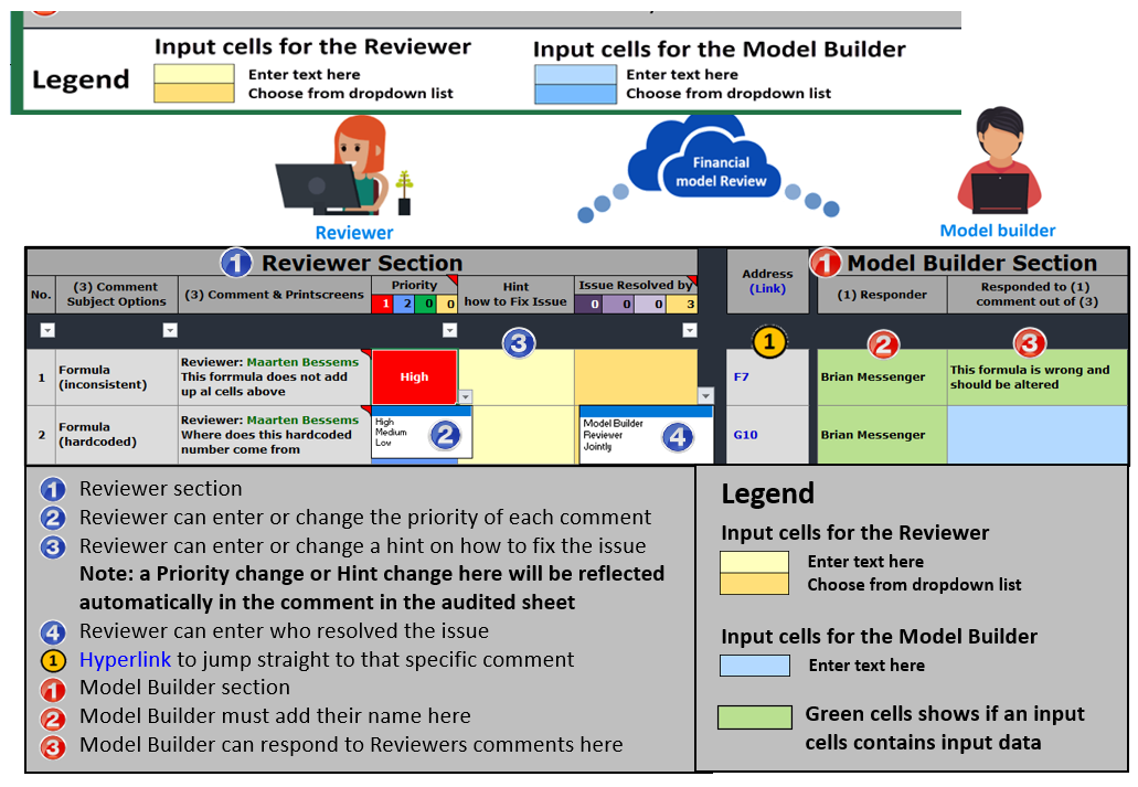
The following on-line help panels explain the different areas of the Comment Feature report:

So now instead of correcting the individual sheets, the Reviewer will use “Tracing formulas” in the Review Panel to identify why the formulas in the F7 and G7 cells are different.

It highlights cell F4 and G4 have been omitted from the SUM functions at F7 and G7. So, since the reviewer cannot make changes in this scenario, a comment will be placed in the sheet below by selecting the faulty formulas and clicking the Add/Edit Comment tab. Which displays the following Comment screen:

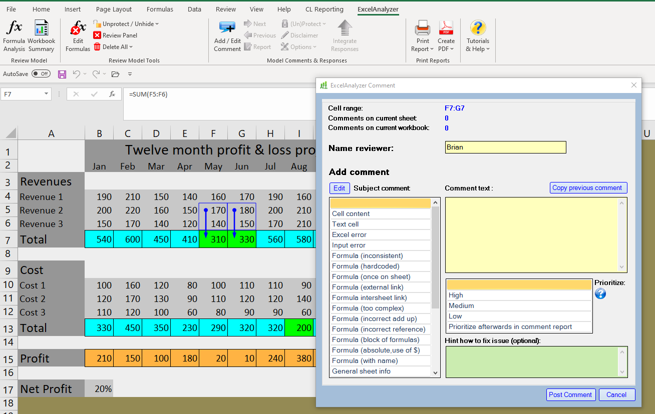
So now, the Reviewer can enter his questions for the Model Builder by selecting a Subject comment from the list or adding one if a relevant one is not listed. Then the Reviewer enters their question as shown, selects a priority and optionally enters a hint on how to fix the issue.

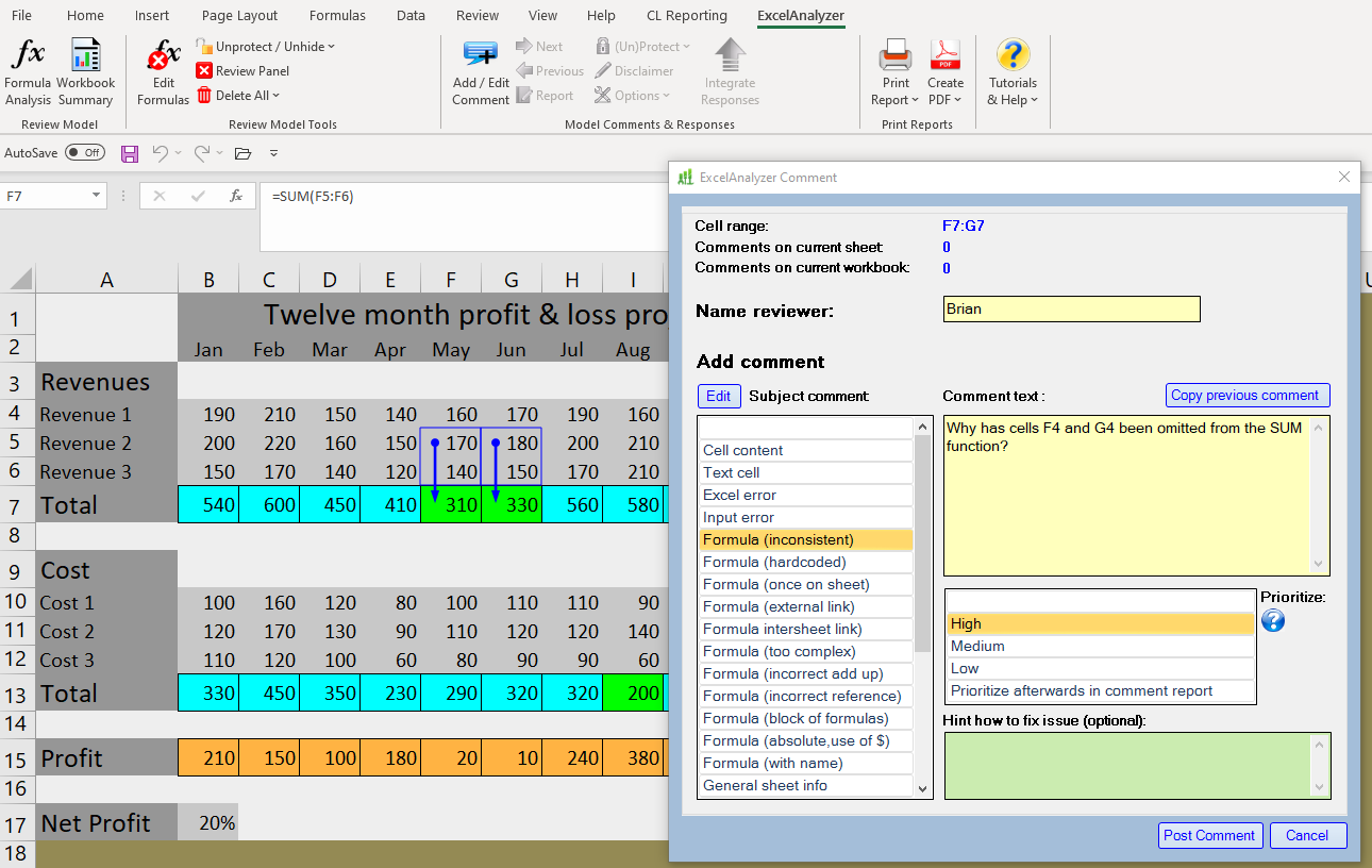
The Reviewer can then click on Post Comment. This results in the Comment information being posted to the faulty formula cells and signified by a red triangle placed at the top right of the first cell in the faulty group selected. If the Reviewer then hovers over the cell with the red triangle, a snapshot of the Comment information will be shown.

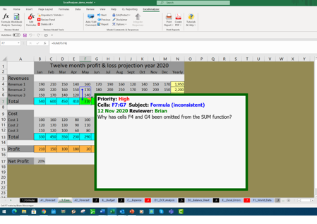
Each of the inconsistencies on this sheet can be Commented and queried in the same way resulting in 3 red triangles. The formula in cell N17 is not inconsistent it is a once on a sheet formula which is given a black background and found to be correct. The sheet name in the sheet ribbon is now suffixed with “_Com” to signify comments present.

The Reviewer now moves onto other sheets and adopts the same process to comment inconsistencies. Once the Reviewer has completed their review, they can optionally cycle through their comments by clicking on the “Next” tab in the Model Comments & Responses section of the ExcelAnalyzer ribbon.

The last step for the Reviewer is to click on the “Report” tab in the Model Comments & Responses section of the ExcelAnalyzer ribbon and then click on the “Start” button.

This generates the Comment Report as an extra tab next to the Formula Report in the sheet ribbon as shown below which shows all of the Reviewer’s comments including the sheet names and cell addresses of the formulas in question.

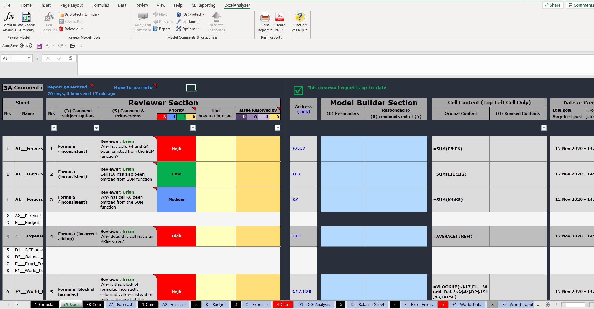
Hovering over each comment in the report will display a printscreen showing the sheet and cells being queried. It also provides an area to the right of the Reviewer’s area which is for the Model Builder to respond to the Reviewer’s queries. This section also provides an address link to the offending cells, the formula in question and the date the comment was posted.

The Reviewer can now send the spreadsheet containing the Comment Reports to the Model Builder who could be a colleague or a Client. As with all of the ExcelAnalyzer reports, the Reviewer could also PDF and/or print the report.

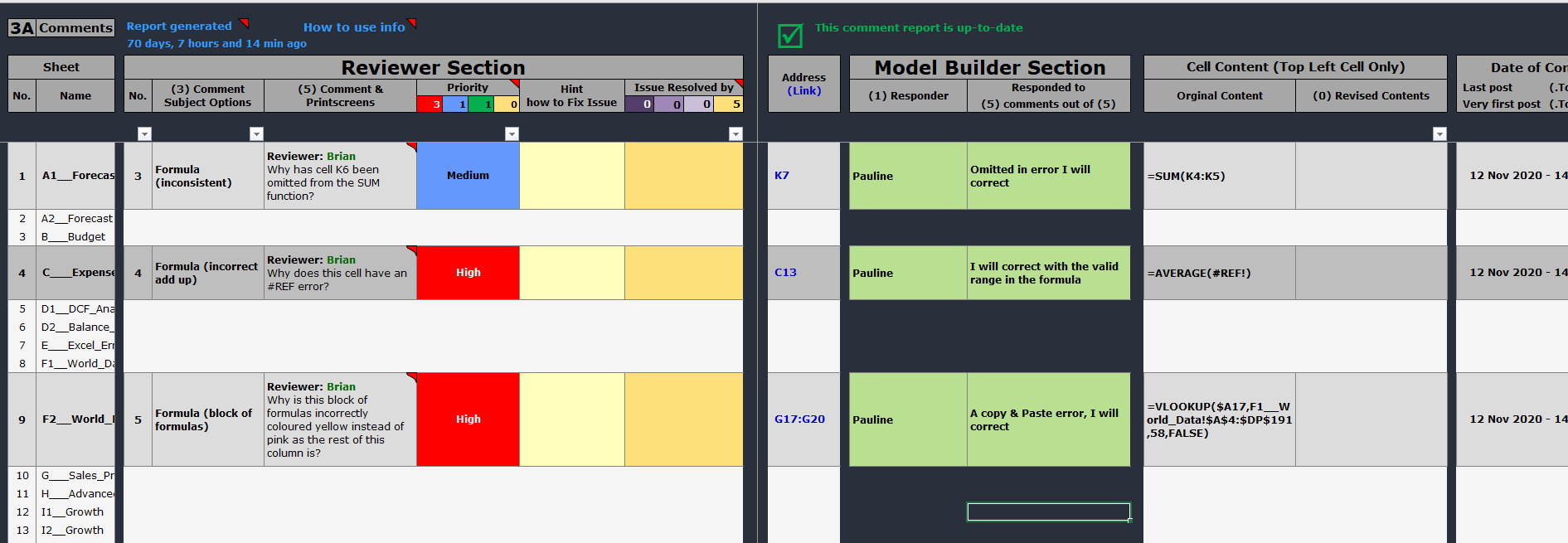
The Model Builder does not need ExcelAnalyzer to be installed to provide the following responses to the Reviewer’s queries. However, ExcelAnalyzer would, of course, enable the Model Builder to build better quality, error-free spreadsheets. Once the Model Builder receives the spreadsheet containing the Comment Report they can respond to the Reviewers queries in the blue section of the report.

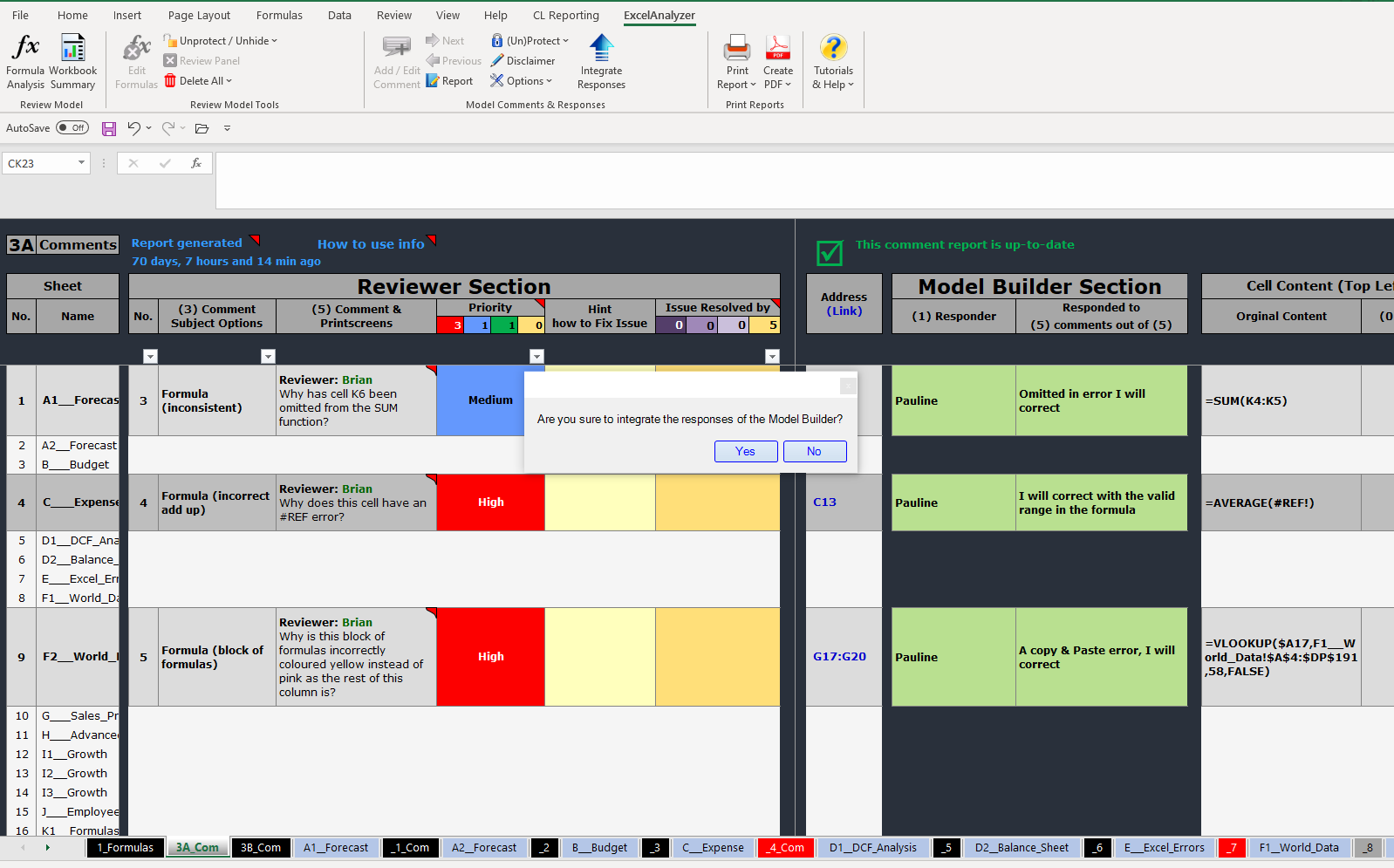
Once the Model Builder has entered her responses, she clicks on the “Integrate Responses” button in the ExcelAnalyzer ribbon to upload the responses their responses into the Comment Report and into the comments on each sheet and clicks “Yes”.

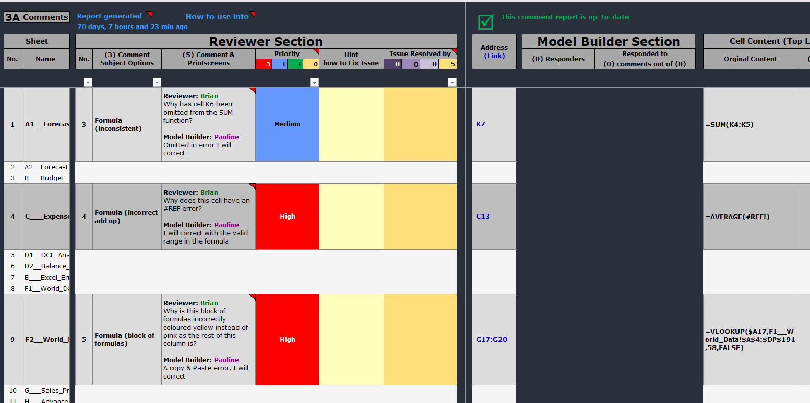
As can be seen below, the responses are now integrated with the Reviewer’s queries. You now have an audit trail report of all queries and responses which can be printed, exported as a PDF and/or saved with this spreadsheet.